Floods are one of the most frequent and devastating natural disasters societies have to cope with. Already in the Epic of Gilgamesh, dating back as far as 2000 BC, the gods flooded the Earth. On the other hand, these ancient civilizations also show that floods are not only bad, they can bring fertility to the land and are part of the natural cycles.
A flood is an inundation occurring in an area that is normally not submerged. One type of flood, the one we predominantly deal with in this article, are river floods (fluvial flood). They occur when the amount of water in a river channel exceeds its holding capacity and spills over into the neighboring land. Currently, each year about 58 million people globally are exposed to river floods and the damage that comes with them, of which more than half live in Asia (simulation by Dottori et al. (2018)). Other types of floods are floods due to excessive rainfall (pluvial floods), or storm surges, where strong winds push sea water onto the coastal areas and inundate them.
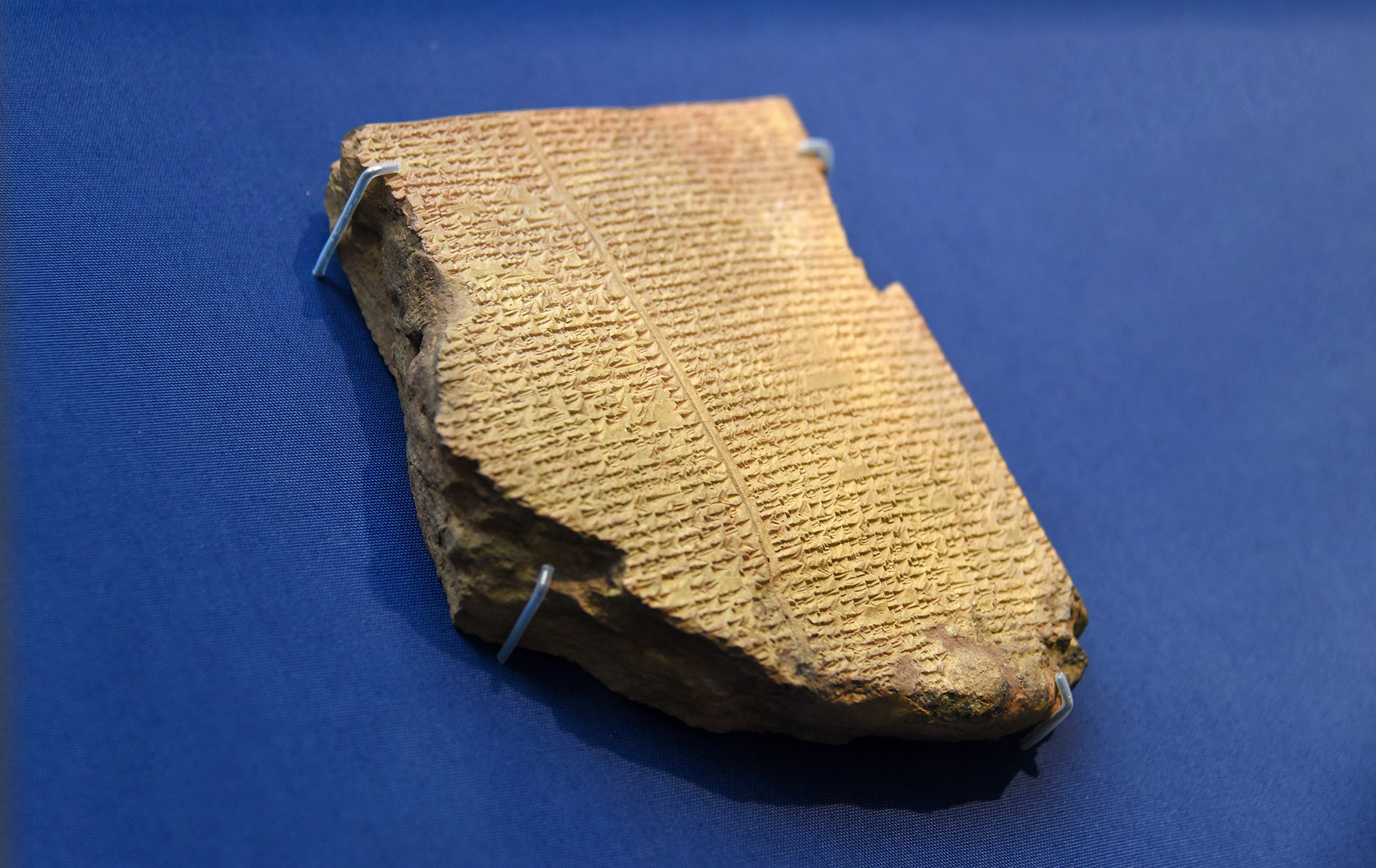
The deluge tablet of the Gilgamesh epic in Akkadian (ca. 1800 BC).
FIG 1 / Image source: Osama Shukir Muhammed Amin
In order to investigate flood events under climate change, a sophisticated tool chain comprising climate models and hydrological models is employed. Hydrological models are our tool to understand how much water flows through a given territory, the consequences of different management options, as well as the potential risks of human settlements near water bodies.
In the following we first describe hydrological processes in general. Then hydrological modelling is discussed, with a particular focus on the model ”CaMa Flood” developed by 山崎大 (Dai YAMAZAKI) at the University of Tokyo (Yamazaki et al. 2011) and applied by Lange et al. (2020) among others.
What makes a flood? - Critical hydrological processes that have to be described when trying to estimate the extent of a flood event
Let’s start at the beginning and then zoom in.
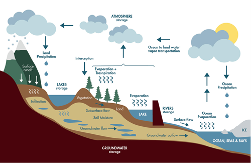
The global water cycle
The (fresh) water’s trajectory on Earth makes up the water cycle, also known as the hydrological cycle.
The water’s journey begins when it evaporates from the oceans’, lakes’ or other water bodies’ surface into the atmosphere. Interestingly, this not only involves a transport of matter, i.e. the water itself, but also the transport of energy. It takes a certain amount of energy to evaporate water, i.e. to change water from its liquid to its gaseous phase. When the water turns back into its liquid phase (condensation) this energy is released as heat again, but quite possibly at a spot far removed from the original place of evaporation. This energy transport is known as latent heat flux.
The water vapor and its stored (latent) heat travel through the atmosphere across the Earth, driven by winds. Eventually some of it comes back down to the Earth’s surface as precipitation, either on the oceans or some other water body, or on land.
These processes, from the evapotranspiration to the precipitation, are simulated within the general circulation models (GCM).
Atmosphere – Land surface interaction – Or where the hydrological model takes over
Precipitation falls onto the land surface as rain or snow. Most of it precipitates onto the land surface, however, a fraction might be intercepted and remain on the leaves of trees or the forest floor, depending on the density of the vegetation canopy. This water store is known as the interception store. From there the water can, for instance, evaporate back into the atmosphere. The amount of water intercepted strongly depends on the vegetation, but can be quite substantial. As an example, for forests in Germany Peck and Mayer (1996) give average values of 21% to 42% of the annual precipitation as intercepted. These numbers depend on the tree species. The interception in a coniferous forest is higher than in a deciduous forest.
A fraction of the water that reaches the ground will remain on the surface, either because the upper soil layer is already saturated with water or because the land surface is impervious (e.g. rock or sealed surfaces as in cities). This surface water either flows onto a pervious piece of land, into the nearest river (surface runoff) or it eventually evaporates. Surface runoff is the fastest runoff component, it takes the shortest amount of time to reach the river system. It is also the runoff component that contributes most to river floods. In a heavy rain event, the top soil layer becomes saturated and therefore additional water cannot trickle into the soil anymore. The soil cannot store any of the pouring rain, and the water flows directly and quickly into the riverbed. If the rain doesn’t stop, the riverbed will not be able to hold all of it and a flood will occur. Rainfall is not the sole cause of river floods, though. Melting snow in spring in the mountains can also be a decisive factor.
However, normally some of the water that reaches the ground trickles into the soil. Here some remains as soil water, some of it is used by the plants via their roots and pumped it back into the atmosphere (transpiration), some percolates into the river system (subsurface runoff), or into an aquifer (groundwater recharge). The groundwater will eventually end up in the river system as well. The subsurface runoff is slower than the surface runoff, and the trickling of the groundwater into the river is the slowest runoff component. The age of groundwater can be thousands of years. Not all of the models handle groundwater explicitly, and for the purposes of flood modelling it typically can be neglected.
Among the different routes that the water might take, the transpiration process is tremendously important, as globally about 60% of the precipitation is pumped back into the atmosphere by the vegetation (Oki and Kanae 2006), and the remaining 40% turns into runoff. Typically, the quantities evaporation and transpiration are combined into the quantity evapotranspiration. Under climate change with its rising temperatures evapotranspiration is generally expected to rise, leading to substantial reductions in the runoff. Consider for instance an annual precipitation of 1000 mm. If the evapotranspiration increases by only 10% (from 600 mm to 660 mm), the runoff already drops by 15% (from 400 mm to 340 mm). These numbers are even more severe in areas with a higher evapotranspiration. This shift in the evapotranspiration–runoff balance is particularly concerning because the runoff is the water that is available to us. In order to give precise numbers for the runoff we would thus not only need sound precipitation estimates, but also precise evapotranspiration numbers. Already our lacking vegetation maps mean that there is still room for improvements. Luckily these mechanisms are not crucial when it comes to river flood modelling.
In mid to high latitudes the water might freeze and it usually remains at its spot until it melts.
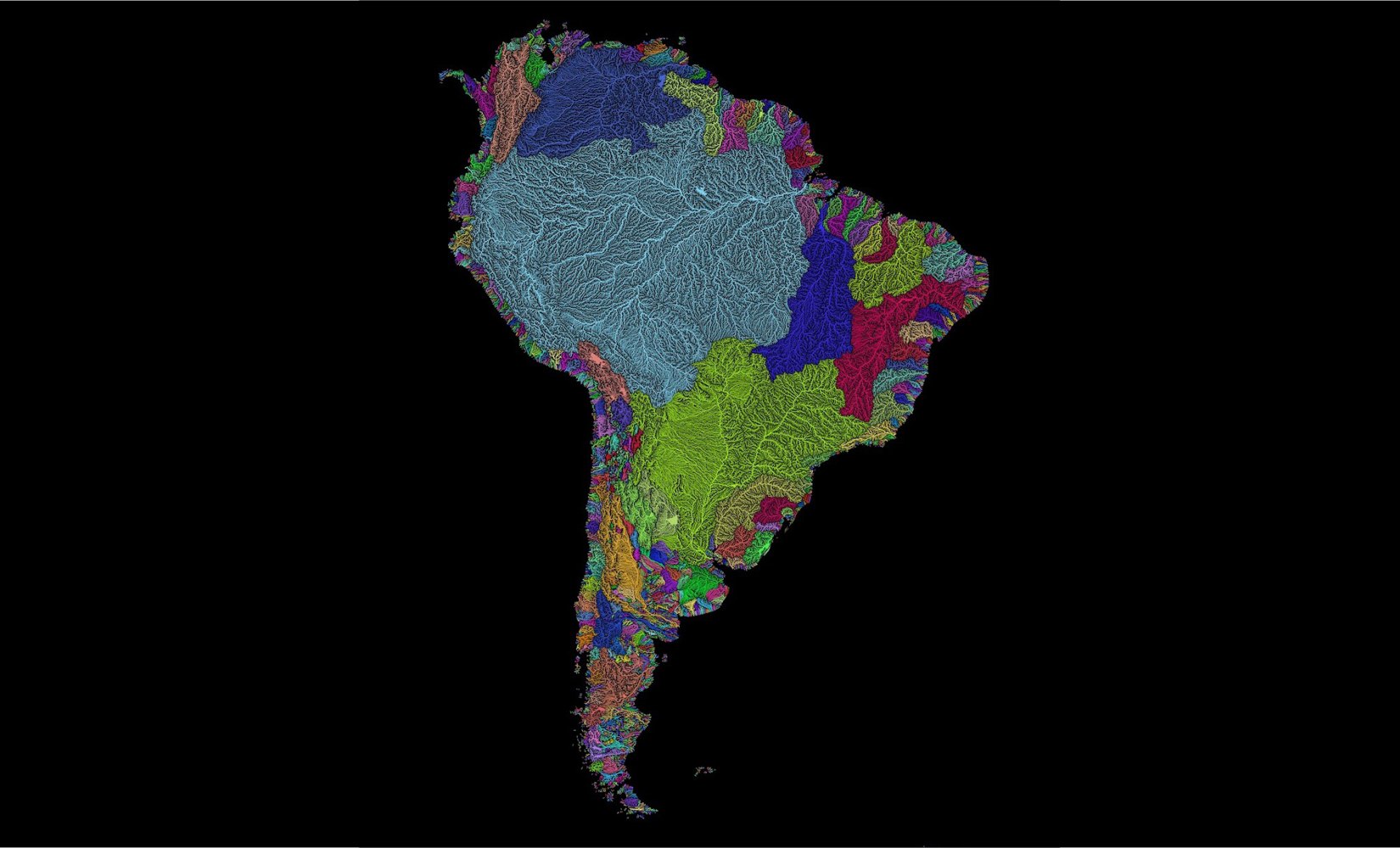
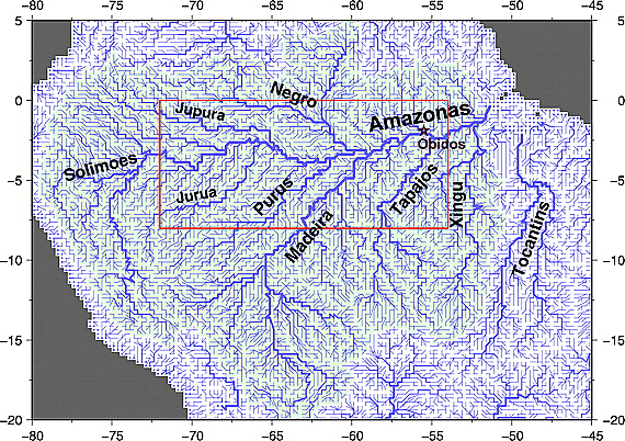
River network and major catchments of South America
FIG 4 / Image source: Robert Szucs(www.grasshoppergeography.com)
Lateral transport of water through river routing
Water is also transported laterally on the Earth’s surface. The Earth’s surface is partitioned into the so-called river basins, also known as river catchments. In a typical basin, all the runoff flows through a river network back into the sea, thereby completing the hydrological cycle. The exact placement of the river reaches and how they connect is mostly determined by the orography of the basin. The water that flows within a river channel is known as the discharge.
Please note that the above outline only gives broad strokes. For instance, precipitation can also be hail, snow/ice can move, as in a glacier, a river does not necessarily flow into the sea (Jordan river) etc.
A part of the South American river network as implemented by CaMa Flood.
FIG 5 / Image source: Yamazaki et al.
Hydrological Modelling
Hydrological models typically implement the atmosphere–land surface interaction and lateral routing.
Hydrological modelling requires an implementation of the discussed processes as well as substantial numerical data to produce reliable simulations. Climate datasets are key input data into hydrological models. A hydrological model requires data such as daily precipitation, temperature (daily average, minimum and maximum), wind and radiation as meteorological input. Furthermore, they also need auxiliary input data such as soil maps providing different soil parameters. This information is necessary to calculate the amount of water that can be stored in a given soil type and thus is available for plants, the different runoff components and so on. Along with the soil data, hydrological models also need to have “an idea” of the vegetation and land use types in the simulated area in order to correctly determine the amount of water that is intercepted and evapotranspired.
Further difficulties lurk in the simulation of the lateral river routing scheme i.e determining the path in which the river flows down to the sea. Hydrological models are often gridded, and the processes described above occur within a grid cell. River routing, on the other hand, transcends a single cell, water is transported from one cell to the next. Figure 5 shows how this is implemented in CaMa Flood. There is a horizontal connection between the grid cells that defines the path in which the water flows from upstream to downstream The routing schemes used within a hydrological model are typically derived from digital elevation maps (DEM), which is a representation of the orography. However deriving the river routing scheme from the DEM can be error prone and often requires manual verification of the routing scheme. Further complications might arise through the grid structure within the model, and so on.
In order to get the water flow through the river system right, the models, in principle, would also need information about the geometry of the river reaches, i.e. its channel width, bank height, roughness, water loss coefficient etc. These parameters, however, are usually not available. In order to still produce reasonable data, these parameters are either determined through simplistic assumptions or by calibration.
Global models usually take the first approach, e.g. the model CaMa Flood discussed below derives the channel width and bank height via a formula from the discharge. Regional models, i.e. models that cover only a single basin at a time, determine these parameters through calibration. In order to calibrate, the model is run many times with different values of the channel width, the bank height, and other parameters, and driven by the observed climate. The parameter set that reproduces the observed discharge the best is then used for the modelling of the basin of interest. Hattermann et al. (2017) contrasts results from global and regional modelling.
Once the parameters have been estimated and/or calibrated, the routing algorithm is ready to determine the water volume in a grid cell’s river reach. Besides the mentioned parameters, it uses the current discharge, the incoming runoff components from the sides and the up- and downstream discharges to calculate the discharge in the next time step. Figure 6 shows an example of a hydrograph, i.e. the discharge at a certain point of a river. More precisely, the discharge of the outlet of the Punpun River Basin in India is displayed. For each month of 1997 the observed (solid line) and the simulated (dashed line) is shown. The model is clearly able to reproduce the main features of the annual cycle with reasonable accuracy.
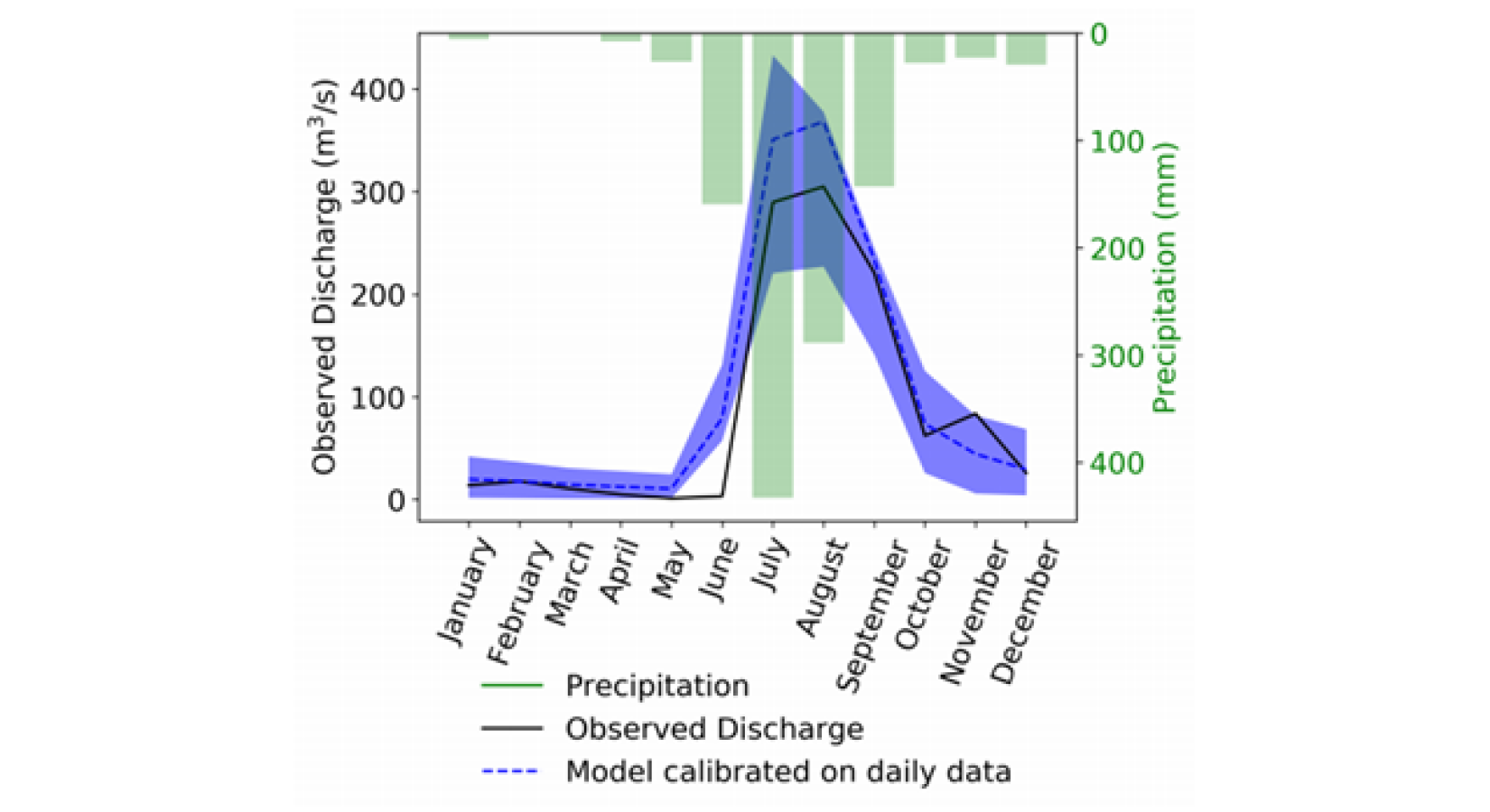
Hydrogram showing the observed and model calibrated monthly river discharge from the Punpun River outlet in India for the year 1997.
FIG 6 / Image source: Adla et al.
Difficulties in Hydrological and Flood Modelling
As explained above, a major problem in hydrological modeling are the uncertainties in the precipitation modeling from the GCMs. Compared to the temperature, precipitation projections are error prone. The modeling chain thus is troubled by uncertainties from the very start. The hydrological models themselves quite often have to wrestle with insufficient input data, for instance the soil, vegetation and land use maps might be lacking in detail. Similarly, data necessary for calibration, might be missing, such as sufficiently long discharge time series. On the other hand, the approaches of the non-calibrating models can be a bit too simplistic for the complex realities they need to describe.
Further difficulties can be encountered outside of the model chain. For future projections, especially the ones about socioeconomic impacts, assumptions about the population, assets and adaptation measures, like increased/decreased flood protection levels have to be made. These assumptions tremendously influence the results, but are only scenarios and might not reflect the future realities.
Flood modelling itself poses its own set of challenges. The basic problem is that detailed flood investigations require an understanding of the flood dynamics. We would like to know where does how much water flow, and with what speeds. The typical time scales and spatial resolutions of the models discussed above cannot provide this information. Their resolution is simply too coarse in every respect. For modeling flash floods, or similarly tsunamis (tsunamis are no river floods) etc, more detailed hydrodynamic models are required. They demand highly precise input, with respect to the water sources as well as the DEM. Typically, in order to investigate such problems, 2D hydrodynamic models are used. Besides the high demands on the input side, they are also computationally expensive and require large computing power. Some applications, such as catastrophic flood modelling has even higher demands. In such applications the modelling “of vertical turbulence, vortices, and spiral flow at bends” (Teng et al. 2017) requires even 3D hydrodynamic models. Such 2D and 3D hydrodynamic simulations are not viable in areas larger than 1000 km2 (Teng et al. 2017).
From runoff to discharge and the extent of flooding – CaMa Flood
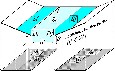
The distinction between the regular river reach (light blue) and the floodplain (dark blue) in CaMa Flood.
FIG 7 / Image source: Yamazaki et Al.
In the following we take a look at a particular hydrological resp. Flood model, “CaMa Flood”. As previously stated, CaMa flood is developed by 山崎大 (Dai YAMAZAKI) and his group at The University of Tokyo. It is a global model and fittingly is used all over the world.
CaMa Flood foregoes the land–surface interaction and concentrates on the lateral transport processes. Therefore it uses runoff generated by other hydrological models as its input.
The name “CaMa Flood” abbreviates the expression “Catchment-based Macro-scale Floodplain model” which hints at its specialty, the sophisticated treatment of floods. Its innovative feature is to explicitly model the floodplain. This is shown in figure 7. Most of the time the water only flows in the normal river channel, depicted in light blue. The channel has the width W and the bank height B. If there is so much discharge, however, that it doesn’t fit into the regular river anymore, the water spills over into the floodplain. This is the water shown in dark blue. By explicitly incorporating floodplain inundation dynamics CaMa Flood strives to improve the predictability of the river discharge and the precision of flood modelling. The water in the floodplain is then put into the context of a DEM, which allows to analyze floods in detail by providing variables such as flood depth Df, flooded area Af and so on.
Sometimes the term “bathtub method” is used for this, because the discharge is simply poured into the DEM and the flood dynamics are ignored. This approach is computationally cheap, though, and therefore CaMa Flood is able to simulate floods on the global scale. Only by using this approach works such as Dottori et al. (2018) and Lange et al. (2020) are possible.
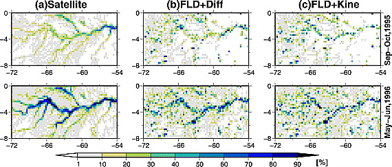
CaMa Flood performance in the Amazon river basin. The top shows the flooded area fraction Sep–Oct 1995 and the bottom shows the flooded area fraction May–June 1996. The left column shows satellite measurements, while the middle and right columns show CaMa Flood simulation. They represent two different calculation schemes in CaMa Flood.
FIG 8 / Image source: Yamazaki et Al.
Figure 8 shows the performance of CaMa Flood in reproducing two flood events. Both occurred in the Amazon basin, the top row shows the months Sep–Oct 1995 and the bottom row the months May–June 1996. The left column shows satellite measurements, the color describes how much of an area is inundated. The middle and the right columns show CaMa Flood simulations of these two events. They differ in the calculation schemes employed. One can see that both calculation schemes roughly reproduce the observation, although in this case the FLD+Diff scheme gives somewhat better results (higher correlations, not discussed here). This illustration should give you a feel for the performance of CaMa Flood.
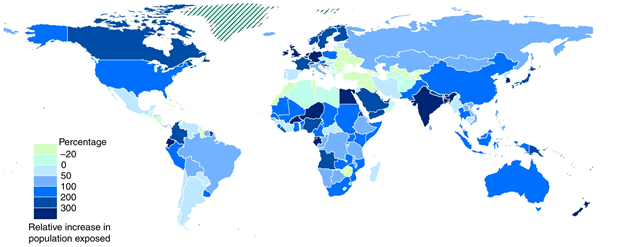
The relative change in the population (SSP5) exposed to river floods in a 3 °C world. The baseline is the 1976 to 2005 period.
FIG 9 / Image source: Dottori et Al.
CaMa Flood is designed to answer a variety of questions regarding river floods. For instance, it was used by Dottori et al. (2018) to investigate “human losses, direct economic damage and subsequent indirect impacts (welfare losses) under a range of temperature (1.5 °C, 2 °C and 3 °C warming).” The researchers used an ensemble of 50 GCM-hydrological model combinations (10 hydrological models each driven by 5 GCM), and fed their runoff into CaMa Flood. Using an ensemble of models instead of a single one allows to estimate the uncertainty of the projections through the model spread. Socioeconomic conditions were taken from SSP3 and SSP5 scenarios. Figure 9 shows the relative change of the population exposed to river floods. More precisely, the map shows the change of a 3 °C and SSP5 world when compared to the baseline. The baseline in this case is the 1976 to 2005 population and its exposure to river floods in that period. In the plot one can see that some countries are projected to be hit particularly hard. For instance, the exposed population in Germany, India, the UK and some other countries is projected to more than triple. Nonetheless, some countries, e.g. in Eastern Europe, are also projected to be less exposed in a hotter world. The analysis assumes present day flood protections levels, i.e. there is no adaptation, and the figure depicts the ensemble mean. For further details we have to refer to the publication.
Another application is the already mentioned impact study by Lange et al. (2020). The results are of course given in the paper, but presentations of the results are also available at this website, here and here.
Conclusions
Millions of people are exposed to river floods. We broadly outlined the hydrological cycle and how it is translated into the model chains used by climate impact researchers. Hydrological models, among them CaMa Flood, are the major tool to investigate changes in frequencies and intensities of river floods under a changing climate and help us make informed decisions about flood protection levels and other adaptation measures.
Acknowledgements
This article was written in collaboration with Katja Frieler, and the ISIpedia Editorial Team.
References
Affiliations
1 Climate Impacts and Vulnerabilities, Potsdam Institute for Climate Impact Research (PIK), 14473 Potsdam, Germany